1 Bioequivalence vs Non-inferiority vs Inferiority

When conducting a clinical trial, a hypothesis of interest needs to be identified and defined. Various statistical techniques can be used to address the chosen hypothesis, depending on the type of comparison that is being made. The most common comparison is between the effects of a new treatment compared to the current treatment. That said, the specific comparison of interest will shape the hypothesis and in turn, the statistical method required.

There are three possible hypothesis that can be formulated when comparing two treatments:

1. The new treatment is at least as effective as the current treatment (non-inferiority)

2. The new treatment is strictly more effective than the current treatment (inferiority)

3. The new treatment is equivalent to the current treatment (bioequivalence)

While these three possible hypothesis appear to be similar, they are slightly different, and thus require slightly different statistical tests.

Non-inferiority trails are used to test whether a minimum level of efficacy has been achieved in the new treatment. These trials are designed to show that the new treatment is no less effective than the existing treatment.

Inferiority/superiority trials are used to test whether the new treatment is strictly more effective than the current treatment. These trials are designed to detect a difference between treatments.

Bioequivalence trials are used to test whether a new treatment is the same, within an acceptable range, to the current treatment. These trials are designed to confirm the absence of a meaningful difference between treatments.

Before we define the hypothesis’ and their corresponding statistical test, it important to identify the type of outcome variable that is of interest.

2 Outcome Variable Type

2.1 Binary Outcome

Unpaired

Non-inferiority:

vs

Inferiority:

vs

Bioequivalence:

vs

and

SAS Code:

data table_unpair;

p1=0.4203;

p2=0.4638;

theta=p1-p2;

n1=69;n2=69;

var=(p1*(1-p1)/n1)+(p2*(1-p2)/n2);

se=sqrt(var);

delta=0.1;

zright=(theta+delta)/se;

zleft=(theta-delta)/se;

pright=1-cdf("normal",zright);

pleft=cdf("normal",zleft);

run;

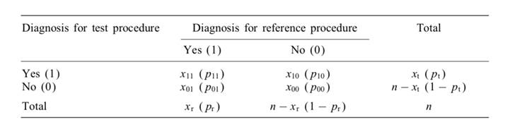
Paired

Non-inferiority:

vs

Inferiority:

vs

Bioequivalence:

versus

and

SAS Code:

data table;

p1=0.4203; *p1=proportion of 1 in protocol 1;

p2=0.4638; *p2=proportion of 1 in protocol 2;

p10=0;

p01=0.0435;

theta=p1-p2;

n=69;

var=(p10+p01-theta*theta)/n;

se=sqrt(var);

delta=0.1;

zright=(theta+delta)/se; *two-tailed test;

zleft=(theta-delta)/se; *two-tailed test;

pright=1-cdf("normal",zright);

pleft=cdf("normal",zleft);

run;

2.2 Continuous Outcome

: treatment score/treatment effect

: reference score/reference effect

: common standard deviation

Unpaired

Non-inferiority:

vs

Inferiority:

vs

Bioequivalence:

vs

and

SAS Code:

data Process;

input _STAT_ $4. @6 Process $3. @10 Quality Yield Waste;

cards;

N New 27 27 27

MEAN New 34.6667 50.0000 11.9889

STD New 1.8605 0.8321 2.2548

N Old 27 27 27

MEAN Old 19.9530 40.1481 10.3556

STD Old 0.8077 0.7698 2.1445

;

proc ttest data=Process sides=L h0=\delta ;

class Process;

var Waste;

run;

Paired

Non-inferiority

vs

Inferiority

vs

Bioequivalence

vs

and

SAS Code:

data Process;

input _STAT_ $4. @6 Process $3. @10 Quality Yield Waste;

cards;

N New 27 27 27

MEAN New 34.6667 50.0000 11.9889

STD New 1.8605 0.8321 2.2548

N Old 27 27 27

MEAN Old 19.9530 40.1481 10.3556

STD Old 0.8077 0.7698 2.1445

;

proc ttest data=Process sides=L h0=\delta ;

class Process;

Paired;

run;

3 Choice of

In the preceding section, a value of is referenced. This value is known as the margin of clinical significance. For a given study, the larger the value of , the bigger the observed difference in treatments needs to be in order to reject the null hypothesis. The choice of largely depends on the context of the particular study. For example, for a study on suicide rate, even a small in reducing the rate of suicide will have a significant impact on the lives of those at risk.

Although there is no general rule on how to specify this margin, it must be specified based on clinical and statistical reasoning; however, it is considered as one of the most challenging steps in the design of these types of trials. Literature suggests that the margin should be defined based on the historical evidence of the active comparator, which is often a well established standard treatment. Often, will be chosen based on a minimally clinically meaningful difference, or a cost-benefit breakpoint.

Often it is sufficient to ask an expert in the appropriate field to provide a margin that is acceptable for the study (Example: 5%, 10%, 15%).

4 References

1. Althunian, T. A., de Boer, A., Groenwold, R. H. H., & Klungel, O. H. (2017). Defining the noninferiority margin and analysing noninferiority: An overview. British Journal of Clinical Pharmacology

2. Committee for Proprietary Medicinal Products. (2001). Points to consider on switching between superiority and non-inferiority. British Journal of Clinical Pharmacology

3. Tsong, Y., Zhang, J., & Levenson, M. (2007). Choice of δ noninferiority margin and dependency of the noninferiority trials. Journal of Biopharmaceutical Statistics

4. Wang, B., Wang, H., Tu, X. M., & Feng, C. (2017). Comparisons of Superiority, Non-inferiority, and Equivalence Trials. Shanghai Archives of Psychiatry