(Time-to-Event)
Survival Analysis
Survival analysis,
also known as time-to-event analysis, refers to the methods of analyzing the
expected time until the occurrence of an event. The time-to-event data records
the time duration from the start of an observation till an event, the end of the
study, lost contact of the participant or withdrawal from the study. Survival
analysis involves modelling the time-to-event data. In the context of survival
analysis, death and failure are considered as an event, and for each
individual the event occurs at most once.
Survival analysis
aims to analyze the patterns of event time and solve the relationship
between explanatory variables and survival time. There are three common
approaches to model the survival function: non-parametric (e.g. Kaplan-Meier
method), semi-parametric (e.g. Cox proportional hazards models) and parametric
(e.g. Weibull model, log-normal model).
Concepts of common terms
The followings are
some common terms in the approaches of survival analysis:
-
Survival function: Probability of surviving past a given time (event-free past
t).
![]()
- Probability
density function: Unconditional probability that event will occur at the exact
time between ![]() and
and ![]() :
:
![]()
- Hazard
function: Instantaneous risk that an event will occur at a given time, given no
event until that time:
![]()
Non-parametric analysis
The most common
non-parametric technique is the Kaplan-Meir (KM) estimator. The KM estimator
breaks the estimation of ![]() into intervals
upon observed event times. Within each interval, the probability of surviving
is calculated, given that the subjects involved are at risk at the beginning of
the time interval.
into intervals
upon observed event times. Within each interval, the probability of surviving
is calculated, given that the subjects involved are at risk at the beginning of
the time interval.
Under this
approach, ![]() is the product
of survival probabilities at each interval until time
is the product
of survival probabilities at each interval until time ![]() .
.
The estimator of
survival probability at each interval is calculated as:

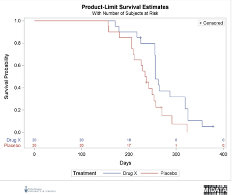
This figure shows an
example of the survival curve calculated from the KM method.
Parametric analysis
Compared to
non-parametric approaches, parametric forms are more informative and have more
statistical power when the models are correctly specified. The hazard function
and the effect of the covariates are defined in parametric approaches, where
the hazard function is the estimation from an assumed distribution in the
underlying population.
Accelerated Failure
Time (AFT) models are a class of parametric survival models that can be linearized
by taking logs of the survival time model. The AFT model is expressed as:
![]() where
where ![]() is the error
term.
is the error
term.
The distributions
that can specify for ![]() and the error
term include:
and the error
term include:
|
Distribution
of |
Distribution
of the error term |
|
Weibull |
Extreme
value (2 parameters) |
|
Exponential |
Extreme
value (1 parameter) |
|
Gamma |
Log
gamma |
|
Log-logistic |
Logistic |
|
Log-normal |
Normal |
Example Code in SAS
/* Parametric
way */
OPTIONS PS=65 LS=100
NODATE NONUMBER ;
DATA HEADACHE ;
INPUT MINUTES GROUP
CENSOR @@ ; DATALINES ;
11 1 0 12 1 0 19 1 0
19 1 0 19 1 0 19 1 0 21 1 0
20 1 0 21 1 0 21 1 0
20 1 0 21 1 0 20 1 0 21 1 0
25 1 0 27 1 0 30 1 0
14 2 0 16 2 0 16 2 0 21 2 0
21 2 0 23 2 0 23 2 0
23 2 0 23 2 0 23 2 0 24 2 0
24 2 0 30 2 0 21 1 1
24 1 1 25 2 1 26 2 1 32 2 1
30 2 1 32 2 1 20 2 1
; RUN ;
PROC LIFEREG DATA
= HEADACHE ;
CLASS GROUP ;
MODEL MINUTES * CENSOR( 1 ) = GROUP ;
RUN ;
/* Non-parametric way
*/
PROC FORMAT ; VALUE RX 1 = "DRUG X" 0
="PLACEBO" ; RUN ;
DATA EXPOSED ; INPUT DAYS STATUS TREATMENT SEX $ @@ ;
FORMAT TREATMENT RX. ; DATALINES ;
179 1 1 F 378 0 1 M
256 1 1 F 355 1 1 M 262 1 1 M
319 1 1 M 256 1 1 F
256 1 1 M 255 1 1 M 171 1 1 F
224 0 1 F 325 1 1 M
225 1 1 F 325 1 1 M 287 1 1 M
217 1 1 F 319 1 1 M
255 1 1 F 264 1 1 M 256 1 1 F
237 0 0 F 291 1 0 M
156 1 0 F 323 1 0 M 270 1 0 M
253 1 0 M 257 1 0 M
206 1 0 F 242 1 0 M 206 1 0 F
157 1 0 F 237 1 0 M
249 1 0 M 211 1 0 F 180 1 0 F
229 1 0 F 226 1 0 F
234 1 0 F 268 0 0 M 209 1 0 F
RUN ;
ODS GRAPHICS ON ;
TITLE1 “ FIRST OF 3 ANALYSES “ ;
PROC LIFETEST DATA =
EXPOSED plots=(survival(atrisk=0
to 1000 by 100 test)
loglogs
logsurv); TIME DAYS * STATUS(0) ; STRATA
TREATMENT ; RUN ;
ODS GRAPHICS OFF ;
Example Code in R
install.packages("survival")
install.packages("ranger")
install.packages("ggplot2")
install.packages("dplyr")
install.packages("ggfortify")
# load librarys
library(survival)
library(ranger)
library(ggplot2)
library(dplyr)
library(ggfortify)
# Non-parametric way
# use
attached dataset cancer
data("cancer")
# Kaplan Meier Analysis
km_fit <- survfit(Surv(time, status) ~ 1, data=cancer)
summary(km_fit)
autoplot(km_fit)
# Semi-parametric way
vet <- mutate(cancer,
AG = ifelse((age < 60), "LT60", "OV60"),
AG = factor(AG))
# Cox proportional hazards model
cox <- coxph(Surv(time,
status) ~ 1, data=vet)
summary(cox)
cox_fit <- survfit(cox)
autoplot(cox_fit)
References
1. Stel
V, S, Dekker F, W, Tripepi G, Zoccali C,
Jager K, J: Survival Analysis I: The Kaplan-Meier Method. Nephron Clin Pract 2011;119:c83-c88. doi:
10.1159/000324758
2. Kartsonaki, C. (2016a). Survival analysis. Diagnostic
Histopathology, 22(7), 263–270. https://doi.org/10.1016/j.mpdhp.2016.06.005.
3. Singh,
R., & Mukhopadhyay, K. (2011). Survival analysis in clinical trials: Basics
and must know areas. Perspectives in clinical research, 2(4), 145–148.
https://doi.org/10.4103/2229-3485.86872
4. Goel,
M. K., Khanna, P., & Kishore, J. (2010). Understanding survival analysis:
Kaplan-Meier estimate. International journal of Ayurveda research, 1(4),
274–278. https://doi.org/10.4103/0974-7788.76794
5. Time-To-Event
Data Analysis. (n.d.). Columbia Public Health. Retrieved November 3, 2021, from
https://www.publichealth.columbia.edu/research/population-health-methods/time-event-data-analysis