ROC and
AUC
Example Codes: R #1 SAS #1 R #2 SAS #2
Contingency Table
A contingency table (also known as a cross
tabulation or crosstab) is a type of table in a matrix format that displays the
(multivariate) frequency distribution of the variables. They provide a basic
picture of the interrelation between two variables and can help find
interactions between them.
In reality, we frequently use it to analyze the
relationship between treatment and event.
|
|
Event |
No Event |
|
Treatment |
a |
b |
|
Control |
c |
d |
Terms Used
Odds Ratio (OR): The odds ratio is the ratio of
the odds of an event in the Treatment group to the odds of an event in the
control group.

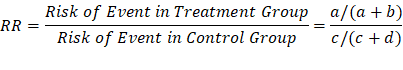
Relative Risk (RR): The relative
risk (RR) of an event is the likelihood of its occurrence after exposure to a
risk variable as compared with the likelihood of its occurrence in a control or
reference group.
Confusion Matrix
A confusion matrix, also known as an error
matrix, is a specific table layout that allows visualization of the performance
of an algorithm. It is a special kind of contingency table, with two dimensions
("actual" and "predicted"), and identical sets of
"classes" in both dimensions (each combination of dimension and class
is a variable in the contingency table).
The Layout of the confusion matrix is as follow:
|
|
|
Predicted Condition |
|
|
|
Total population = P + N |
Positive (PP) |
Negative (PN) |
|
Actual condition |
Positive (P) |
True Positive (TP) |
False Negative (FN) |
|
Negative (N) |
False Positive (FP) |
True Negative (TN) |
|
1.
True Positive (TP): A test result
that correctly indicates the presence of a condition or characteristic.
2.
True Negative (TN): A test result
that correctly indicates the absence of a condition or characteristic.
3.
False Positive (FP): A test result
which wrongly indicates that a particular condition or attribute is present.
4.
False Negative (FN): A test result
which wrongly indicates that a particular condition or attribute is absent.
Terms Used
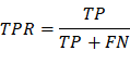
TPR/Sensitivity: True positive rate, measures
the proportion of positives that are correctly identified(correctly
identify those with a disease).
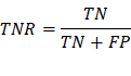
TNR/Specificity: True negative rate,
measures the proportion of negatives
that are correctly identified (correctly identify
those without a disease).
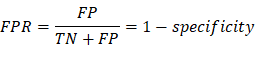
FPR/Type I Error: False positive
rate, measures the proportion of negatives that are wrongly categorized as
positives. (The probability of rejecting the null hypothesis when it’s true)
FNR/Type II Error: False negative
rate, measures the proportion of positives that are wrongly categorized as
negatives. (The probability of accepting the null hypothesis when it’s false)

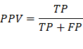
PPV/Precision: Positive predictive value,
the probability that following a positive test result, that individual will
truly be positive.
NPV: Negative predictive value, the probability
that following a negative test result, that individual will truly be negative.

R Example
#Install required packages
install.packages('caret')
install.packages('epitools')
#Import required library
library(caret)
#Creates vectors having data
points
expected_value <- factor(c(1,0,1,0,1,1,1,0,0,1))
predicted_value <- factor(c(1,0,0,1,1,1,0,0,0,1))
#Creating confusion matrix
example <- confusionMatrix(data=predicted_value, reference = expected_value)
#Display results (including
Sensitivity, Specificity, PPV, NPV)
example
#Simpler way - confusion matrix
alone
tab = table(expected_value,predicted_value)
tab
# OR and RR
epitools::oddsratio(tab, method = 'wald')
epitools::riskratio(tab, method = 'wald')
SAS Example
data predicts;
input expect predict;
datalines;
1 1
0 0
1 0
0 1
1 1
1 1
1 0
0 0
0 0
1 1
;
proc
freq data=predicts;
tables expect*predict / chisq relrisk senspec;
run;
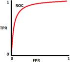
ROC and AUC
The ROC curve (relative operating characteristic curve) is a
probability curve created by plotting the TPR (sensitivity) against FPR (1-specificity)
at various thresholding with FPR on the x axis and TPR on the y axis. It is a
performance measurement for the classification problems.
AUC (area under the ROC curve) represents the degree or measure of
separability. It measures the model’s capability of distinguishing between
classes. The higher the AUC, the better the model is to classify 0 classes as 0
and 1 classes as 1(separability).
Interpretation:
-
AUC close to 1: The model has a good measure of
separability, indicating a perfect model to distinguish between
positive(disease) and negative(no-disease) classes.
-
AUC close to 0: The model has really bad
separability. Moreover, it is identifying 0 classes as 1 and 1 classes as 0.
-
AUC = 0.5: the model has no capacity to separate classes, the prediction will be close to random guess.
-
AUC = 0.8, there is a 80
percent chance for the model to correctly distinguish between classes
In general, a rule of thumb of interpreting the
accuracy from AUC and ROC is that a test with an area greater than 0.9 has high
accuracy, while 0.7–0.9 indicates moderate accuracy, 0.5–0.7, low accuracy and
0.5 a chance result.
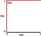
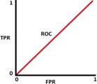
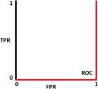
AUC = 1 AUC = 0.5 AUC = 0 AUC = 0.8
R Example
library(ROCR)
library(mlbench)
# recoding the
categorical variables into class 1 and class 0
data(BreastCancer)
df = data.frame(BreastCancer)
df$type <- ifelse (df$ Class ==
"benign", 1, 0)
#build training
and test sets from the dataset
index = sample(1 : nrow(df), size = 0.6 * nrow(df))
train = df[index,
]
test = df[-index,]
#fitting a
logistic regression model
model = glm(type
~ Cell.size + Cell.shape + Epith.c.size, data=train,
family = binomial(link
= "logit"))
#predicting the
test data
pred = predict(model, test, type="response")
pred = prediction(pred, test$type)
#plotting ROC
roc = performance(pred, "tpr",
"fpr")
plot(roc, colorize = T, lwd = 2)
abline(a = 0, b
= 1) #calculating AUC
auc = performance(pred,
measure = "auc")
auc@y.values
SAS Example
data roc;
input alb tp totscore popind @@;
totscore = 10 - totscore;
datalines;
3.0 5.8 10 0 3.2 6.3 5 1 3.9 6.8 3 1 2.8 4.8 6 0
3.2 5.8 3 1 0.9 4.0 5 0 2.5 5.7 8 0 1.6 5.6 5 1
3.8 5.7 5 1 3.7 6.7 6 1 3.2 5.4 4 1 3.8 6.6 6 1
4.1 6.6 5 1 3.6 5.7 5 1 4.3 7.0 4 1 3.6 6.7 4 0
2.3 4.4 6 1 4.2 7.6 4 0 4.0 6.6 6 0 3.5 5.8 6 1
3.8 6.8 7 1 3.0 4.7 8 0 4.5 7.4 5 1 3.7 7.4 5 1
3.1 6.6 6 1 4.1 8.2 6 1 4.3 7.0 5 1 4.3 6.5 4 1
3.2 5.1 5 1 2.6 4.7 6 1 3.3 6.8 6 0 1.7 4.0 7 0
3.7 6.1 5 1 3.3 6.3 7 1 4.2 7.7 6 1 3.5 6.2 5 1
2.9 5.7 9 0 2.1 4.8 7 1 2.8 6.2 8 0 4.0 7.0 7 1
3.3 5.7 6 1 3.7 6.9 5 1 3.6 6.6 5 1
;
ods graphics on;
proc logistic data=roc plots(only)=roc;
LogisticModel: model popind(event='0') = alb tp totscore;
output out=LogiOut predicted=LogiPred; /* output predicted value, to be used later */
run;
References
Karimollah H.T(2013) Receiver Operating Characteristics(ROC) Curve Analy-
sis for Medical Diagnostic Test Evaluation. Caspian J Intern Med 2013
Spring;4(2) 627-635 https://cran.r-project.org/web/packages/ROCR/ROCR.pdf
Anthony K Akobeng(2007) Understanding diagnostic tests 3: receiver operating characteristic
curves https://doi.org/10.1111/j.1651-2227.2006.00178.x