Binary

Example Codes:

Comparison: SAS #1 Comparison: R #1 Comparison: SAS #2 Comparison: R #2

Prediction: SAS #1 Prediction: R #1 Prediction: SAS #2 Prediction: R #2


Objectives

If your response variable is binary and you want to analyze the relationship between the binary variable and other variables, logistic regression can deal with that.


Assume the binary variable, y, only contains two values; 0 and 1.


Here is the logistic regression’s expression:


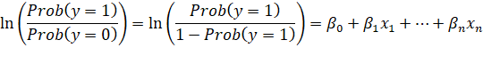
So, the outcome of logistic regression is the probability of getting the response variable equal to 1.


The   is the odds ratio.


General Example Code in SAS

PROC LOGISTIC DATA=SAS-data-set ;

CLASS variables ;

MODEL response=predictors ;

UNITS independent1=list;

ODDSRATIO <label> variable ;

OUTPUT OUT=SAS-data-set keyword=name ;

RUN;


CLASS names the classification variables to be used in the analysis. The CLASS statement must precede the MODEL statement. By default, these variables will be analyzed using effects coding parameterization. This can be changed with the PARAM= option.

MODEL specifies the response variable and the predictor variables.

OUTPUT creates an output data set containing all the variables from the input data set and any requested statistics.

UNITS enables you to obtain an odds ratio estimate for a specified change in a predictor variable. The unit of change can be a number, standard deviation (SD), or a number times the standard deviation (for example, 2*SD).

ODDSRATIO produces odds ratios for variables even when the variables are involved in interactions with other covariates, and for classification variables that use any parameterization. You can specify several ODDSRATIO statements.


Outputs

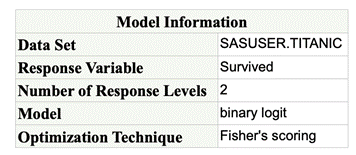
The Model Information table describes the data set, the response variable, the number of response levels, the type of model, the algorithm used to obtain the parameter estimates, and the number of observations read and used.

 Table

Description automatically generated


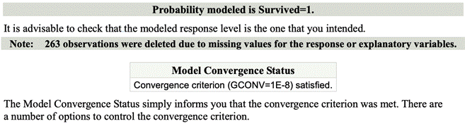
The Number of Observations Used is the count of all observations that are nonmissing for all variables specified in the MODEL statement. The ages of 263 of these 1309 passengers cannot be determined and cannot be used to estimate the model.

 Text

Description automatically generated


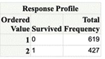
The Response Profile table shows the response variable values listed according to their ordered values. By default, PROC LOGISTIC orders the response variable alphanumerically so that it bases the logistic regression model on the probability of the smallest value. Because you used the EVENT=option in this example, the model is based on the probability of surviving (Survived=1). The Response Profile table also shows frequencies of response values.

 Table

Description automatically generated


 Table

Description automatically generated


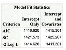
The Model Fit Statistics provides three tests

1.     AIC is AkaikeA’ information criterion.

2.     SC is the Schwarz criterion.

3.     -2 Log L is -2 times the natural log of the likelihood.

-2 Log L, AIC, and SC are goodness-of-fit measures that you can use to compare one model to another. These statistics measure relative fit among models, but they do not measure absolute fit of any single model. Smaller values for all of these measures indicate a better fit.

 Table

Description automatically generated


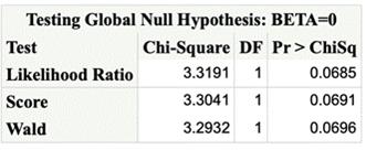
The Testing Global Null Hypothesis: BETA=0 table provides three statistics to test the null hypothesis that all regression coefficients of the model are 0.

 Table

Description automatically generated


The Analysis of Maximum Likelihood Estimates table lists the estimated model parameters, their standard errors, Wald Chi-Square values, and p-values.

 Table

Description automatically generated

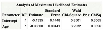
 This information can be expressed in the below equation:


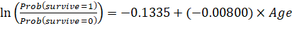
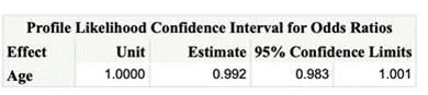
The Wald chi-square and its associated p-value test whether the parameter estimate is significantly different from 0. For this example, the p-values for the variable Age are not significant at the 0.05 significance level (p=0.0696). It cannot be concluded that Age is not important in a multivariate model. The odds ratio and confidence interval can be found in the following table:

Text, table

Description automatically generated with medium confidence


Multinomial


Objectives

If your response variable is multinomial and you want to analyze the relationship between the multinomial variable and other variables, you may use multinomial logistic regression.


Multinomial logistic regression predicts the probability that the response variable  falls into th category. If there are  outcomes for the response variable , then the whole model can be defined as a set of  binary logistic regression. Suppose you have observed data , and fitted coefficients . The following equation represents the th logistic model for predicting the probability of the th outcome. If outcome  (the last outcome) is chosen as the pivot:

Where:

Prediction: Example Code in SAS

data travel;

input AutoTime PlanTime TranTime Age Sex Chosen $;

datalines;

10.0 4.5 10.5 32 1 Plane

5.5 4.0 7.5 13 1 Auto

4.5 6.0 5.5 41 1 Transit

3.5 2.0 5.0 41 1 Transit

1.5 4.5 4.0 47 1 Auto

10.5 3.0 10.5 24 1 Plane

7.0 3.0 9.0 27 1 Auto

9.0 3.5 9.0 21 1 Plane

4.0 5.0 5.5 23 1 Auto

22.0 4.5 22.5 30 0 Plane

7.5 5.5 10.0 58 0 Plane

11.5 3.5 11.5 36 0 Transit

3.5 4.5 4.5 43 0 Auto

12.0 3.0 11.0 33 0 Plane

18.0 5.5 20.0 30 0 Plane

23.0 5.5 21.5 28 0 Plane

4.0 3.0 4.5 44 0 Plane

5.0 2.5 7.0 37 0 Transit

3.5 2.0 7.0 45 0 Auto

12.5 3.5 15.5 35 0 Plane

1.5 4.0 2.0 22 0 Auto

;


proc logistic data = travel;

class chosen;

model chosen = age / link = glogit;

run;


Prediction: Example Code in R

install.packages("nnet")

library(nnet)


travel = data.frame(

AutoTime = c(10,5.5,4.5,3.5,1.5,10.5,7,9,4,22,7.5,11.5,3.5,12,18,23,4,5,3.5,12.5,1.5),

PlanTime = c(4.5,4,6,2,4.5,3,3,3.5,5,4.5,5.5,3.5,4.5,3,5.5,5.5,3,2.5,2,3.5,4),

TranTime = c(10.5,7.5,5.5,5,4,10.5,9,9,5.5,22.5,10,11.5,4.5,11,20,21.5,4.5,7,7,15.5,2),

Age = c(32,13,41,41,47,24,27,21,23,30,58,36,43,33,30,28,44,37,45,35,22),

Sex = c(rep("female",10), rep("male",11)),

Chosen = c("Plane", "Auto", "Transit", "Transit", "Auto", "Plane", "Auto", "Plane", "Auto",

"Plane", "Plane", "Transit", "Auto", "Plane", "Plane", "Plane", "Plane",

"Transit", "Auto", "Plane", "Auto")

)


test <- multinom(Chosen ~ Age, data = travel)

summary(test)


# Predicted probability

head(pp <- fitted(test))

Prediction: Example Code in SAS

data titanic;

set "C:\path\titanic"; /* insert correct path to file here */

run;

proc logistic data=titanic alpha=.05 plots(only)=(effect oddsratio);

model Survived(event='1')=Age / clodds=pl;

run;


Prediction: Example Code in R

# Loading data

mydata <- read.csv("https://web.stanford.edu/class/archive/cs/cs109/cs109.1166/stuff/titanic.csv")

## view the first few rows of the data

head(mydata)


# Train test split

mydata$Survived <- factor(mydata$Survived)

train = mydata[1:700,]

test = mydata[701:887,]


# Fitting model

mylogit <- glm(Survived ~ Age, data = train, family = "binomial")

summary(mylogit)


# Prediction

pred_data = predict(mylogit, newdata = test, type = "response")

## Accuracy:

sum(ifelse(pred_data > 0.5, 1, 0) == test$Survived)/length(test$Survived)


Comparison: Example Code in SAS

The data needed in this code can be downloaded here

data titanic;

set "C:\path\titanic"; /* insert correct path to file here */

run;

proc logistic data=titanic alpha=.05 plots(only)=(effect oddsratio);

class female / param=reference;

model Survived(event='1')=Age female / clodds=pl;

run;


Comparison: Example Code in R

# Loading data

mydata <- read.csv("https://web.stanford.edu/class/archive/cs/cs109/cs109.1166/stuff/titanic.csv")

## view the first few rows of the data

head(mydata)


# Fitting model

mydata$Survived <- factor(mydata$Survived)

mylogit <- glm(Survived ~ Age + Sex, data = mydata, family = "binomial")

summary(mylogit)


Comparison: Example Code in SAS

data travel;

input AutoTime PlanTime TranTime Age Sex Chosen $;

datalines;

10.0 4.5 10.5 32 1 Plane

5.5 4.0 7.5 13 1 Auto

4.5 6.0 5.5 41 1 Transit

3.5 2.0 5.0 41 1 Transit

1.5 4.5 4.0 47 1 Auto

10.5 3.0 10.5 24 1 Plane

7.0 3.0 9.0 27 1 Auto

9.0 3.5 9.0 21 1 Plane

4.0 5.0 5.5 23 1 Auto

22.0 4.5 22.5 30 0 Plane

7.5 5.5 10.0 58 0 Plane

11.5 3.5 11.5 36 0 Transit

3.5 4.5 4.5 43 0 Auto

12.0 3.0 11.0 33 0 Plane

18.0 5.5 20.0 30 0 Plane

23.0 5.5 21.5 28 0 Plane

4.0 3.0 4.5 44 0 Plane

5.0 2.5 7.0 37 0 Transit

3.5 2.0 7.0 45 0 Auto

12.5 3.5 15.5 35 0 Plane

1.5 4.0 2.0 22 0 Auto

;


proc logistic data = travel;

model chosen = age Sex / link = glogit;

run;


Comparison: Example Code in R

install.packages("nnet")

library(nnet)


travel = data.frame(

AutoTime = c(10,5.5,4.5,3.5,1.5,10.5,7,9,4,22,7.5,11.5,3.5,12,18,23,4,5,3.5,12.5,1.5),

PlanTime = c(4.5,4,6,2,4.5,3,3,3.5,5,4.5,5.5,3.5,4.5,3,5.5,5.5,3,2.5,2,3.5,4),

TranTime = c(10.5,7.5,5.5,5,4,10.5,9,9,5.5,22.5,10,11.5,4.5,11,20,21.5,4.5,7,7,15.5,2),

Age = c(32,13,41,41,47,24,27,21,23,30,58,36,43,33,30,28,44,37,45,35,22),

Sex = c(rep("female",10), rep("male",11)),

Chosen = c("Plane", "Auto", "Transit", "Transit", "Auto", "Plane", "Auto", "Plane", "Auto",

"Plane", "Plane", "Transit", "Auto", "Plane", "Plane", "Plane", "Plane",

"Transit", "Auto", "Plane", "Auto")

)


test <- multinom(Chosen ~ Age + Sex, data = travel)

summary(test)